
The Challenge
The 2016 VAST Challenge, MC2 required the analysis of sensor data that detected movement of people q and environmental conditions within zones of multi-storey building. The objective was to identify routine and suspicious behaviour from the spatio-temporal patterns in movement and environment.
This page provides details of the giCentre's solution to the challenge, which won the award 'Outstanding Presentation of Patterns in Context'.
Team Members: Jo Wood
Tools Used: Bespoke software designed and built using Processing, the giCentre Utils library written by the giCentre at City University London and Apache Commons Math library for clustering. Some additinoal minor file processing using Microsoft Excel.
How many hours spent working on submission: Approximately 7 person-days to design and develop the software; 1.5 person-days of analysis and 1.5 person days for writing up and creating the video.
Slides from VIS2016 presentation in Baltimore.
A short paper Visual Analytic Design for Contextualising Sensor Data outlines some of the design challenges for this kind of problem and the video below show the software we built to help answer the challenge questions.
Challenge Questions
MC2.1 What are the typical patterns visible in the prox card data? What does a typical day look like for GAStech employees?
To view the prox card data, the static and mobile prox readings were combined and displayed on a timeline spanning 31st May-13th June. Readings were combined where there were card replacements for an individual employee allowing a single row per person. The employee name and role is indicated on the left hand side of Figure 1.
Each prox card reading is symbolised by a vertical coloured bar positioned according to the time of the reading and coloured by a user-selectable classification. Estimated location is shown as an interpolated horizontal bar between adjacent prox card readings. This provides an overview of each employee's estimated location.
Figures 1 and 2 show each employee's location classified as either in the prox zone of their office (pink) or outside of their office prox zone (blue). These sequences are clustered (using multi-K means++ clustering) to group employees by similar behaviour (each separated by a vertical space) and ordered by cluster size then employee role.
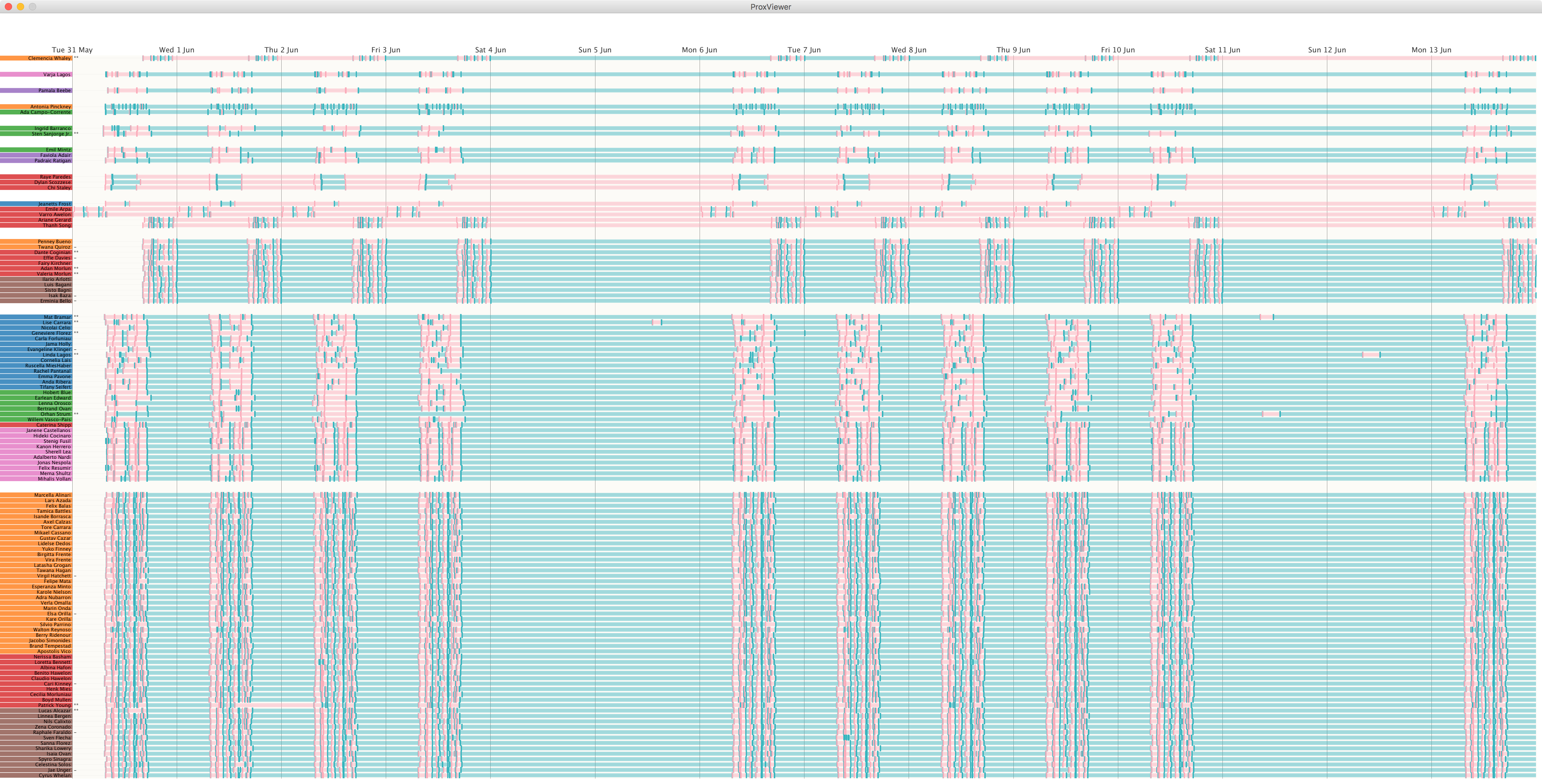
Figure 1: Timelines of prox card entries for each GASTech employee. (click image for full size)

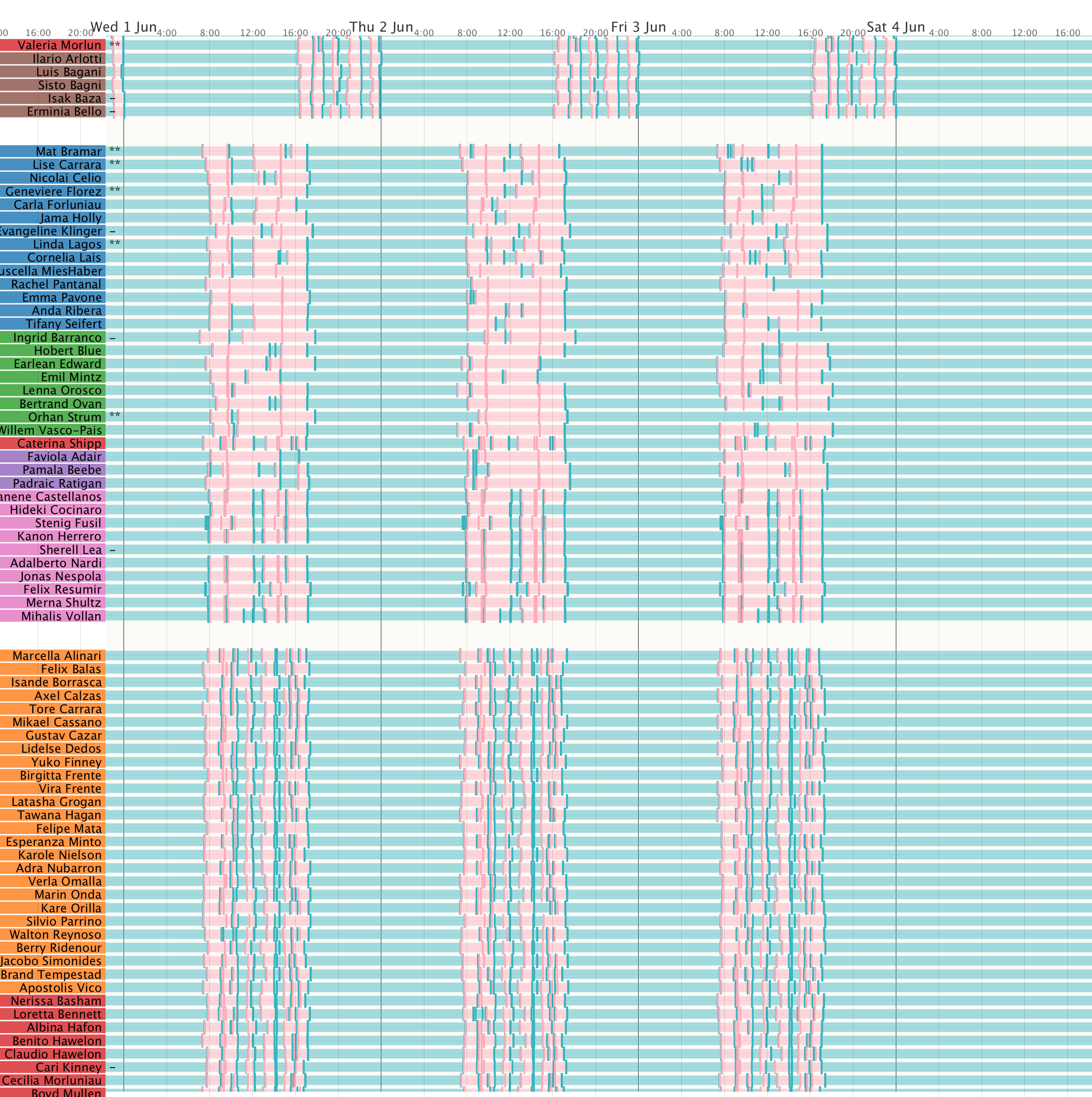
Figure 2. Zoomed in detail of prox card entry view showing typical patterns during the day. Employees symbolised with a '–' indicate note attached to their record and '**' a note with an alert identifying issue of concern. (click image for full size).
This shows that the majority of employees arrive around 8am on weekdays and leave around 5pm. Most employees do not enter the building during weekends. Some, mostly from facilities and IT, work a later shift from 4pm to midnight (as evidenced by the 3rd cluster from bottom in Figure 1) while a couple of others (in 8th cluster from top in Figure 1) work the early shift from midnight to 8am.
To show typical working patterns in more detail, the same layout is applied but classified and clustered according to the function of each prox zone (e.g. office zone, stair/elevator zone, deli zone etc.). This is shown in Figure 3. Where a zone comprises more than one function, its colour is interpolated between the two most dominant functions (e.g. a combined office and meeting zone is a blue-purple hue) giving an indication of uncertainty in behaviour prediction.
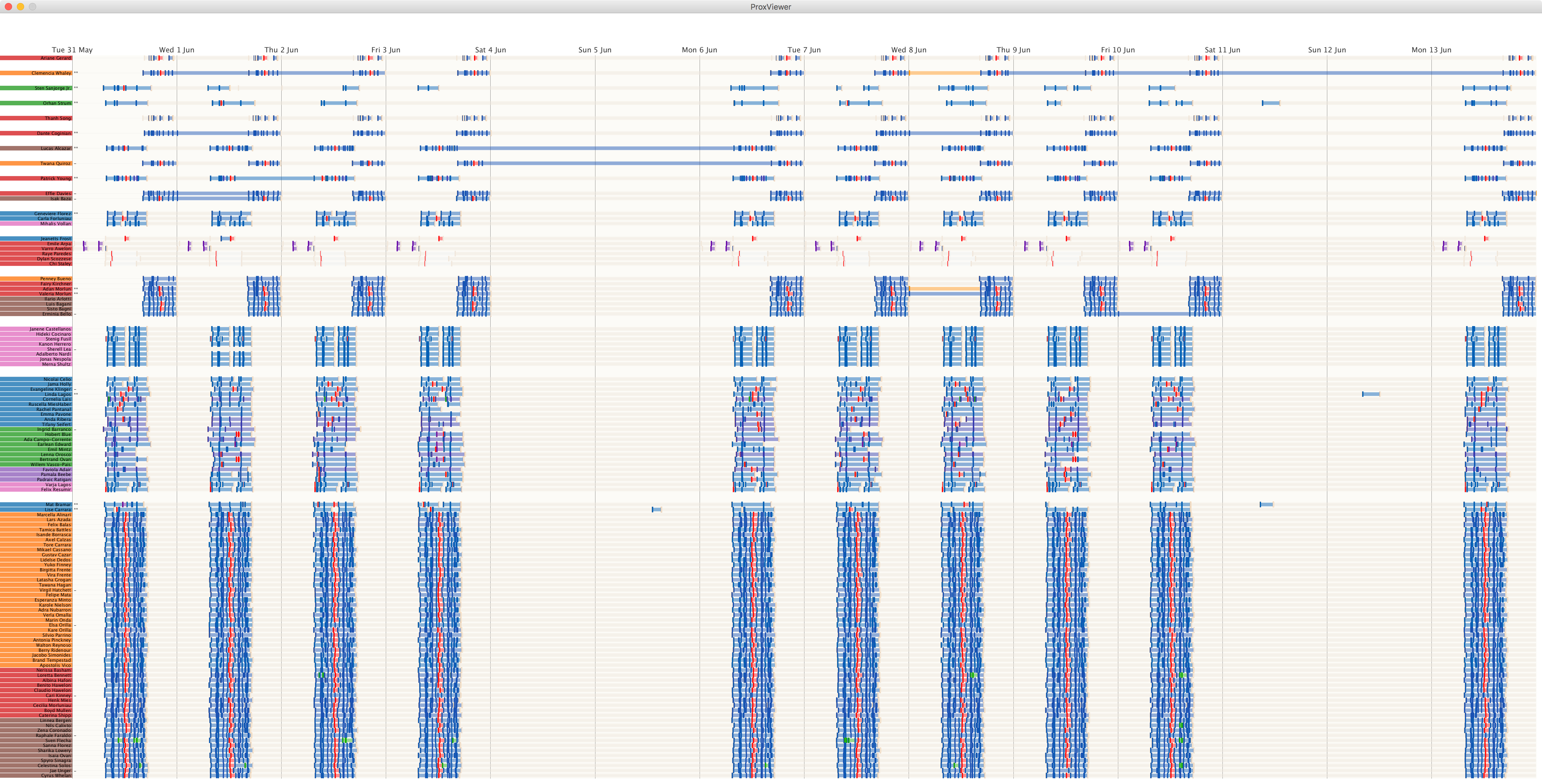
Figure 3 Prox card timelines classified by function of prox zone. (click image for full size)

Most employees (especially in Engineering, Facilities and IT) have their lunch break in the deli (shown in red). This typical pattern can be shown for any single employee as a timeline split by day. Figure 4 below shows the pattern of Virgil Hatchett representing a typical deli-eating day shift employee.
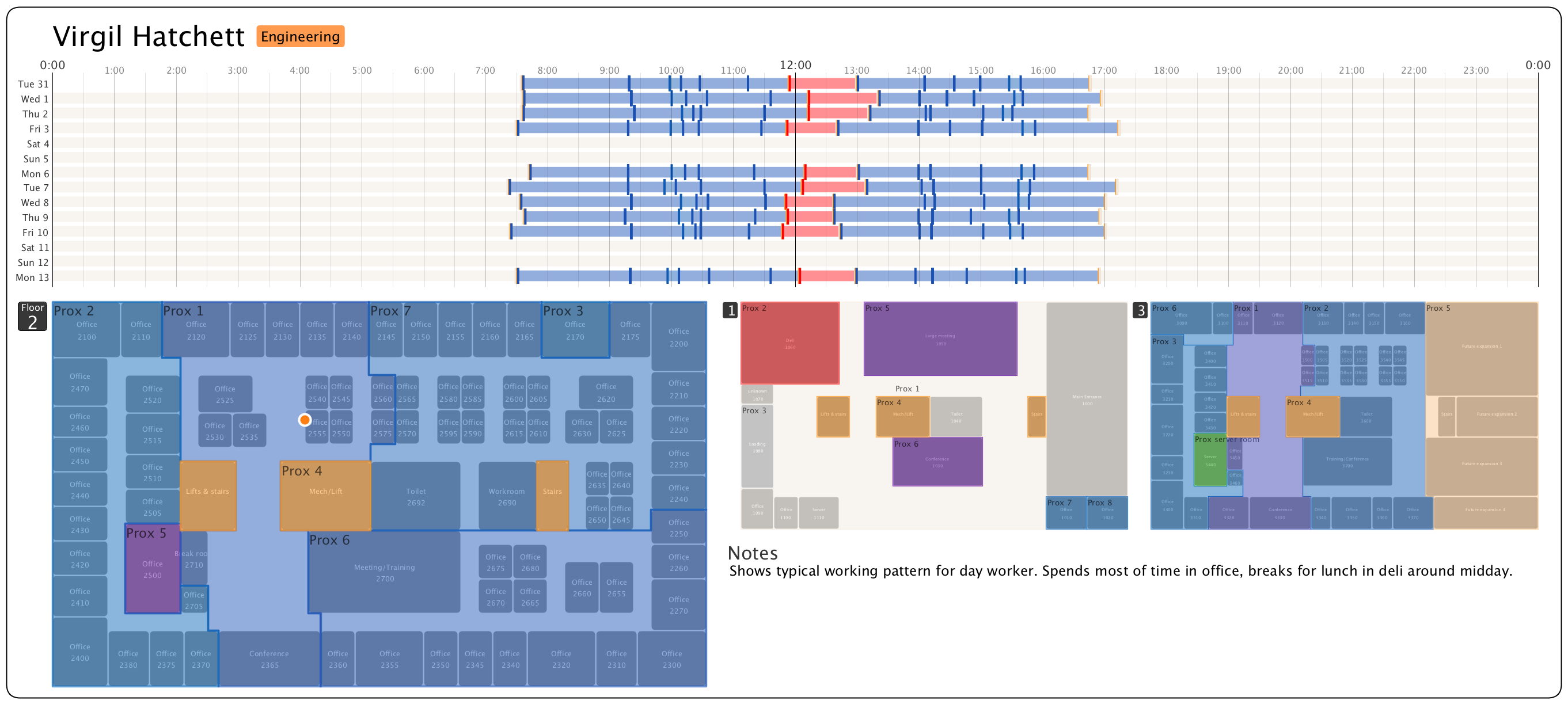
Figure 4 Detail of typical day shift employee pattern classified by prox zone function. (click image for full size)
A similar but later behaviour is exhibited by those on the late shift (e.g. cluster 13 in Figure 3 above and shown for a typical late shift worker in Figure 5 below).
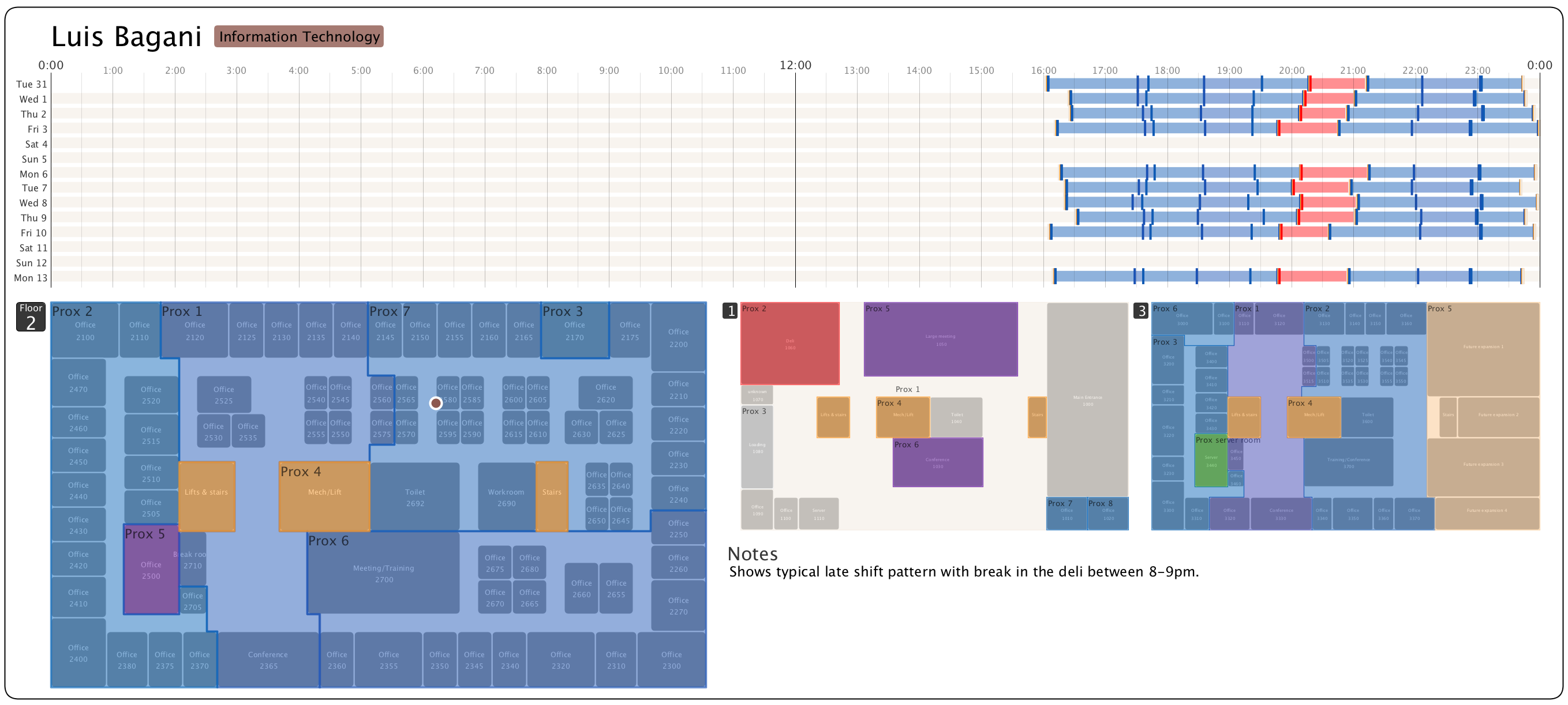
Figure 5 Detail of typical pattern shown by a late shift employee who eats in the deli. (click image for full size)
There is a group of security staff who typically do not eat in the deli but do have a routine period around midday where they are not in their office zone. These are indicated in pink as cluster 14 in Figure 3 and shown for a typical security employee in Figure 6. Most of the executive staff do not eat lunch in the deli but instead stick to locations on the third floor over midday.
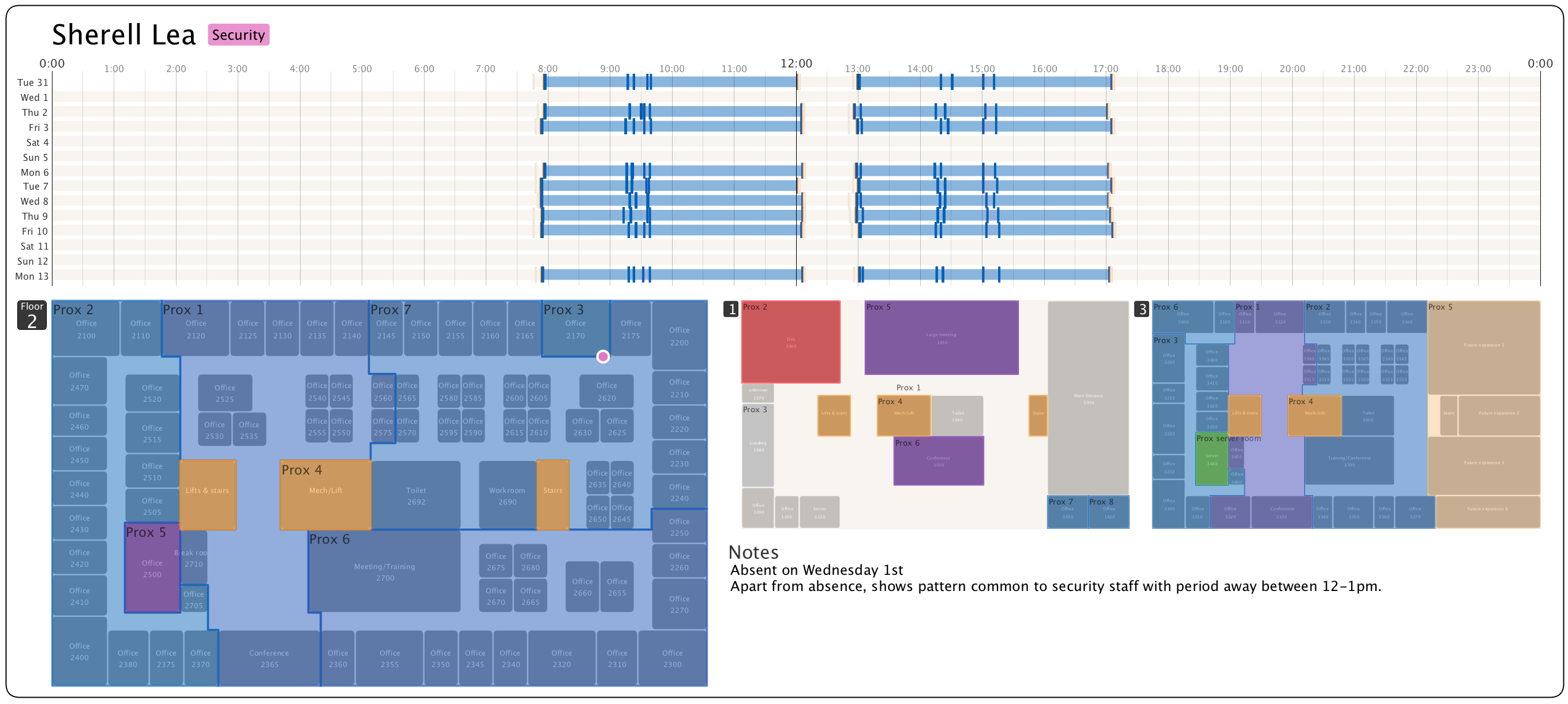
Figure 6 Detail of typical security employee pattern classified by prox zone function. (click image for full size)
MC2.2— Describe up to ten of the most interesting patterns you observe in the building data. Describe what is notable about the pattern and explain what you can about the significance of the pattern.
All 391 HVAC sensors that show some variation between 31st May and 13th of June can be displayed on a timeline and filtered by group, floor or HVAC zone. They can be displayed as raw sensor values, CUSUM charts (used for early live detection of deviation from predicted behaviour), or as z-scores (deviation from mean value normalised by standard deviation). Lines are coloured by floor (red for floor 1, blue for floor 2 and green for floor 3).
(i) Hazium Sensors
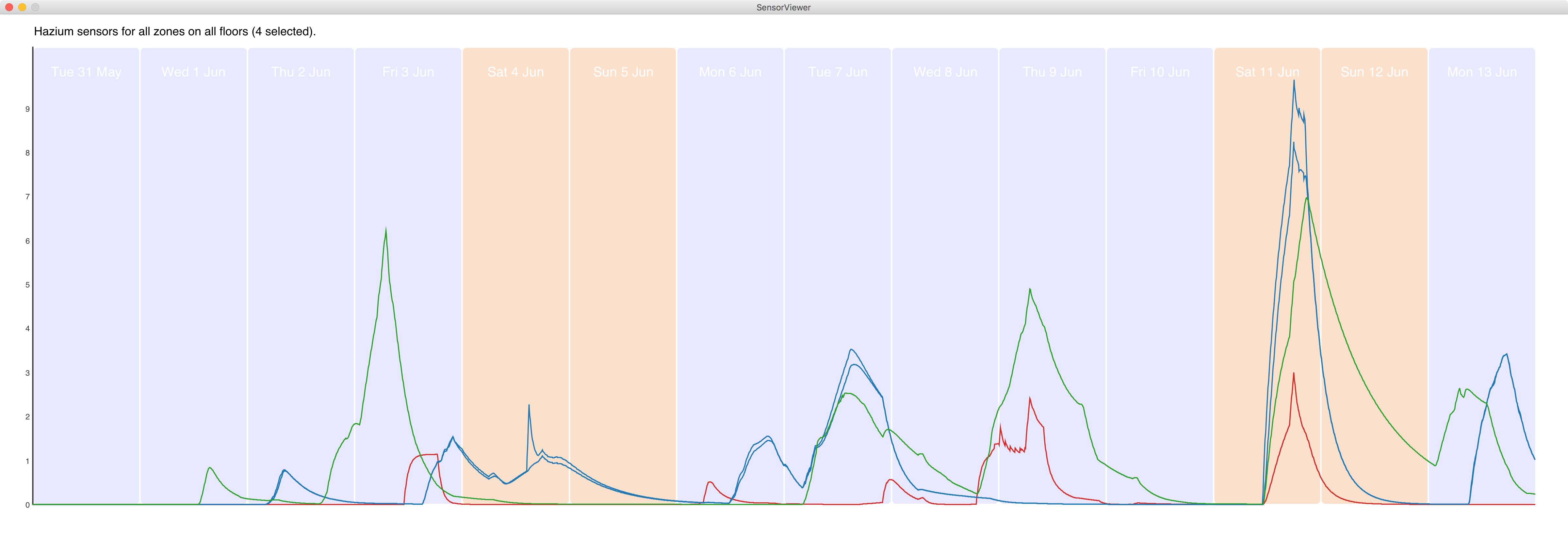
Figure 7 Hazium sensor readings. Scaled by absolute sensor value. Coloured by floor of sensor (floor 1=red; floor 2=blue; floor 3=green; unspecified location = grey). Click image for full size
Potentially harmful Hazium levels are shown to peak on several occasions, notably Friday 3rd on floor 3 and to a slightly lesser extent on floors 1 and 2; Tuesday 7th on floors 2 and 3; Thursday 9th on floors 1 and 3; reaching peak levels on all three floors on Saturday 11th; and a final peak on floors 2 and 3 on Monday 31st. There is some significance in the fact that floor 3 is most commonly affected, possibly due to the nature of the gas (lighter than air?), or due to the source of the leak. There appears to be no unique association with the air and temperature anomalies described below which occur on Tuesday 7th and Wednesday 8th June. There are two peaks on these two days affecting floor 2 in two HVAC zones and floor 3, but they are not confined to these days with larger peaks on other days.
(ii) Carbon dioxide sensors
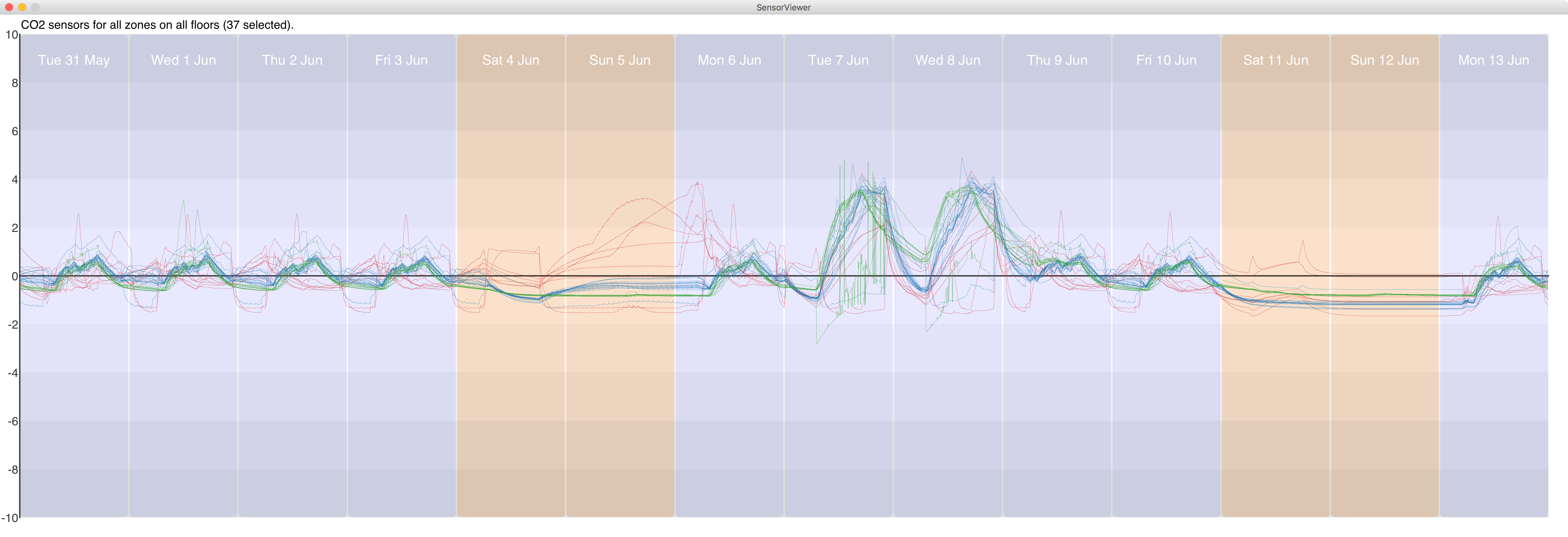
Figure 8 Carbon dioxide sensor readings. Scaled by +- 10 standard deviations from the mean reading. Coloured by floor of sensor (floor 1=red; floor 2=blue; floor 3=green; unspecified location = grey) Click image for full size
Two notable peaks in Carbon Dioxide levels are observed during Wednesday 7th June and Thursday 8th across all floors. This coincides with a major event evident in most sensor readings over these two days. Additionally we see a peak in floor 1 CO2 return outlet concentrations in zones 2,3 and 4 on Sunday 5th June into Monday 6th (red lines).
(iii) Air Flow Sensors
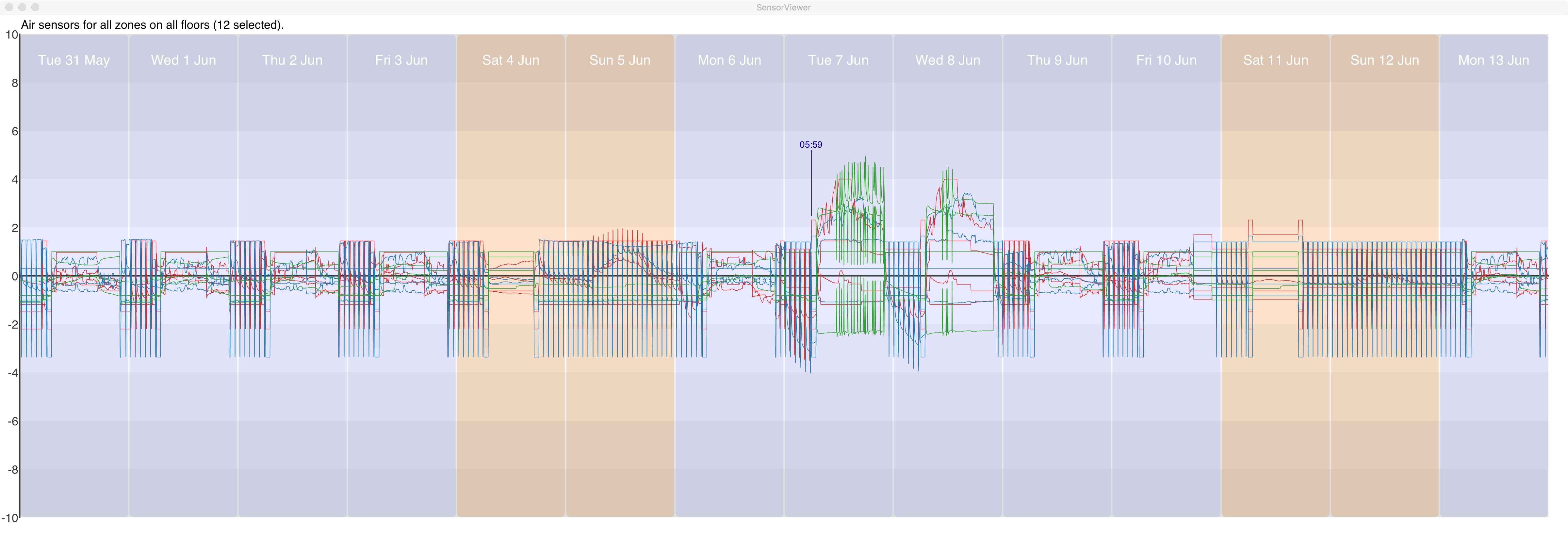
Figure 9 Air flow sensor readings. (click image for full size)
Coinciding with the CO2 peak most of the air flow sensors show anomalies starting at around 7am on Thursday 7th June lasting for two days. Particularly affected are the VAV air loop inlet temperatures, especially for floor 3 (green).
(iv) Variable Air Volume (VAV) Sensors
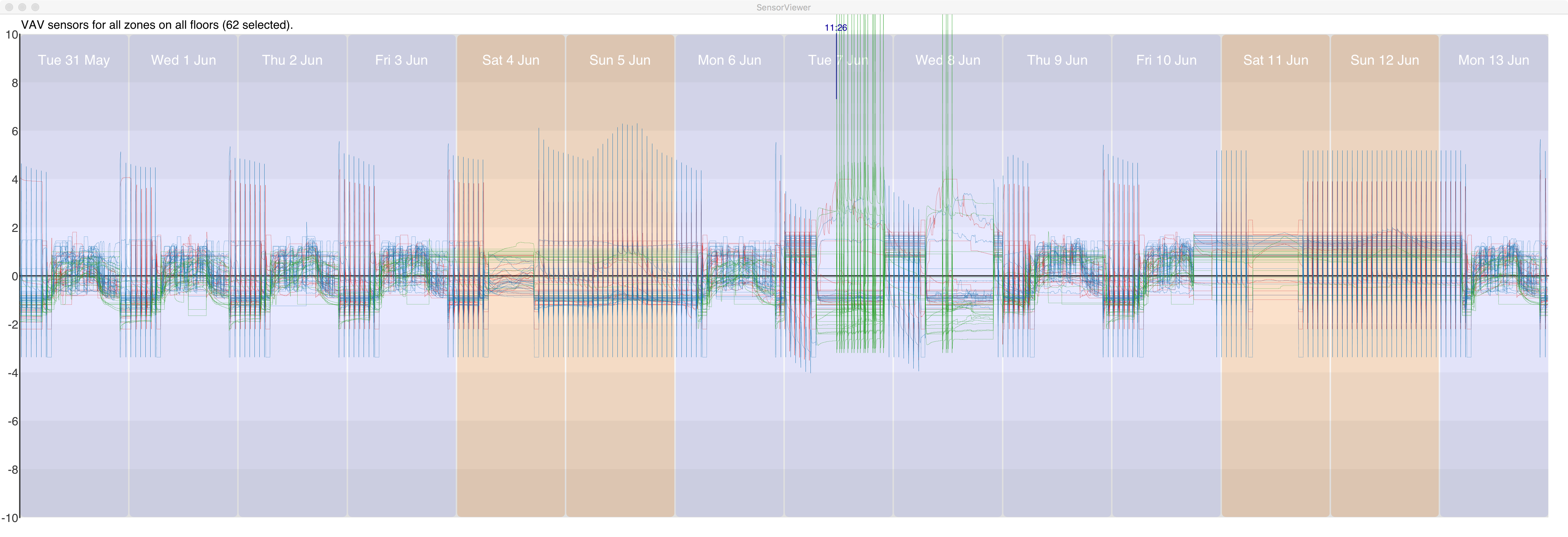
Figure 10 VAV sensor readings. (click image for full size)
The variable air volume (VAV) readings, are dependent, as many others, on occupancy of the building. They show daily fluctuations and weekend/weekday variation. The air and temperature events of the 7th and 8th of June are evident but show a VAV response at around 11:30am which is around 4 hours after the initial air flow anomalies.
(v) Temperature Sensors
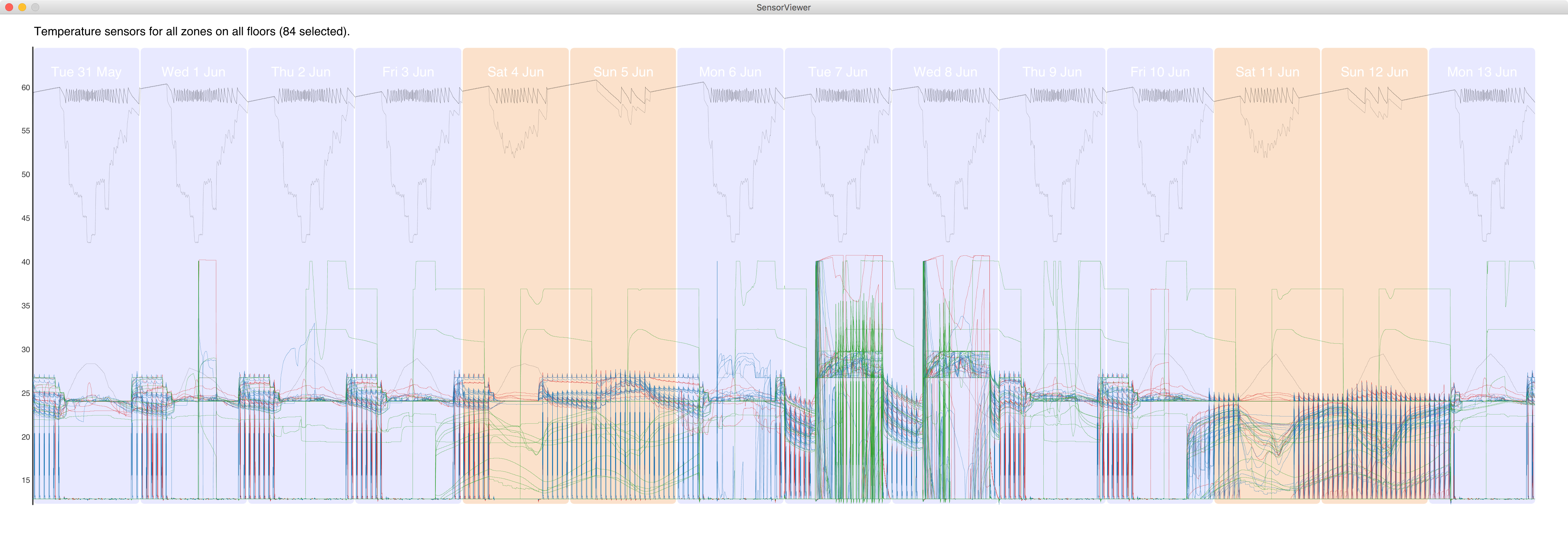
Figure 11a Raw temperature sensor readings. (click image for full size)
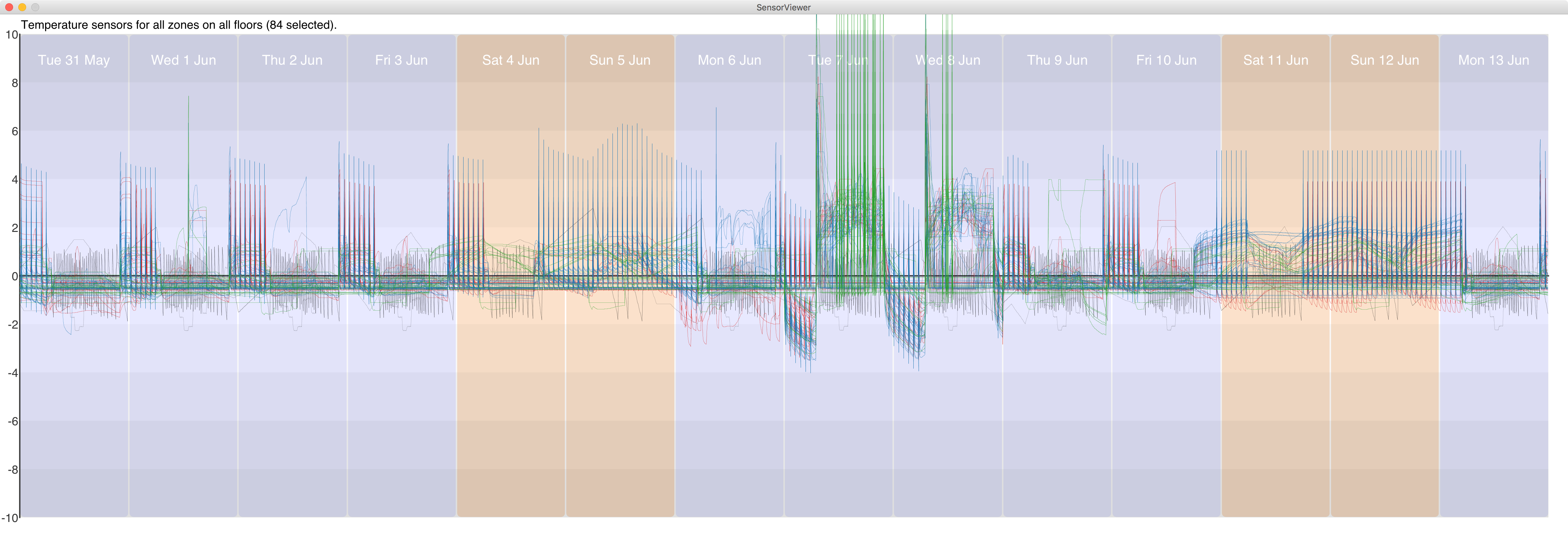
Figure 11b z-score temperature sensor readings (standard deviations from mean). (click image for full size)
The two days associated with the air anomalies are also associated with major temperature changes. The two peaks in temperature, especially on floor 3 on 7th and 8th June, are preceded by a drop in temperature between midnight and 6am. Water temperature and supply side inlet temperature (grey lines at top of Figure 11a) are unaffected by this anomaly.
(vi) Thermostat Sensors
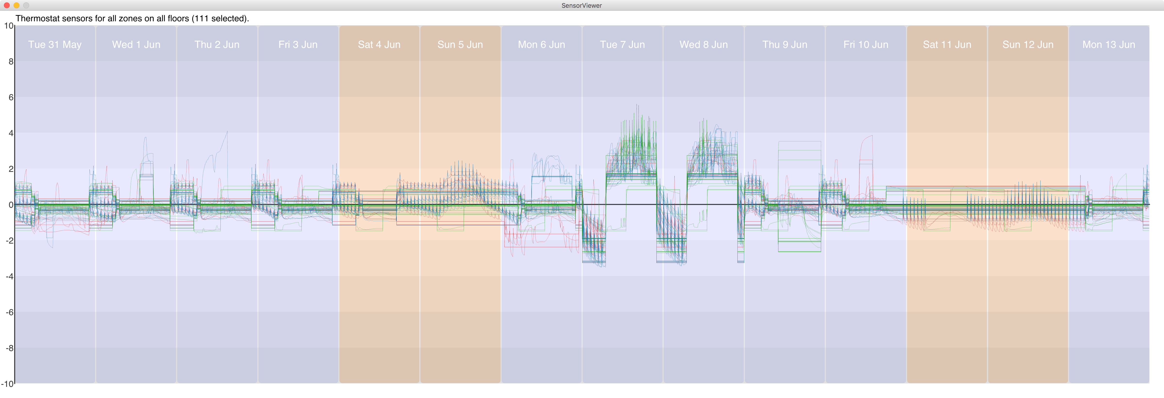
Figure 12 Thermostat sensor readings. (click image for full size)
The temperature fluctuations identified above are also reflected in the thermostat readings that oscillate wildly over the same two days. Additionally, they are preceded by unusually low readings on floor 1 during Monday 6th (red lines).
(vii) Power Sensors
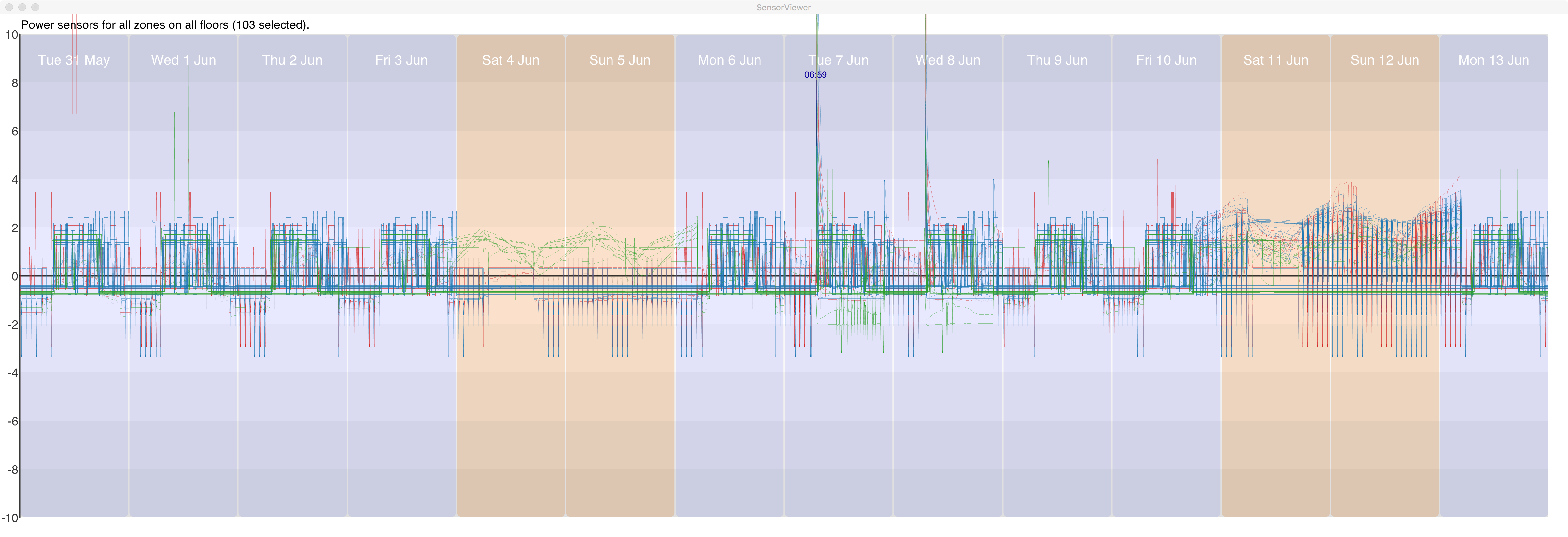
Figure 12 Power sensor readings. (click image for full size)
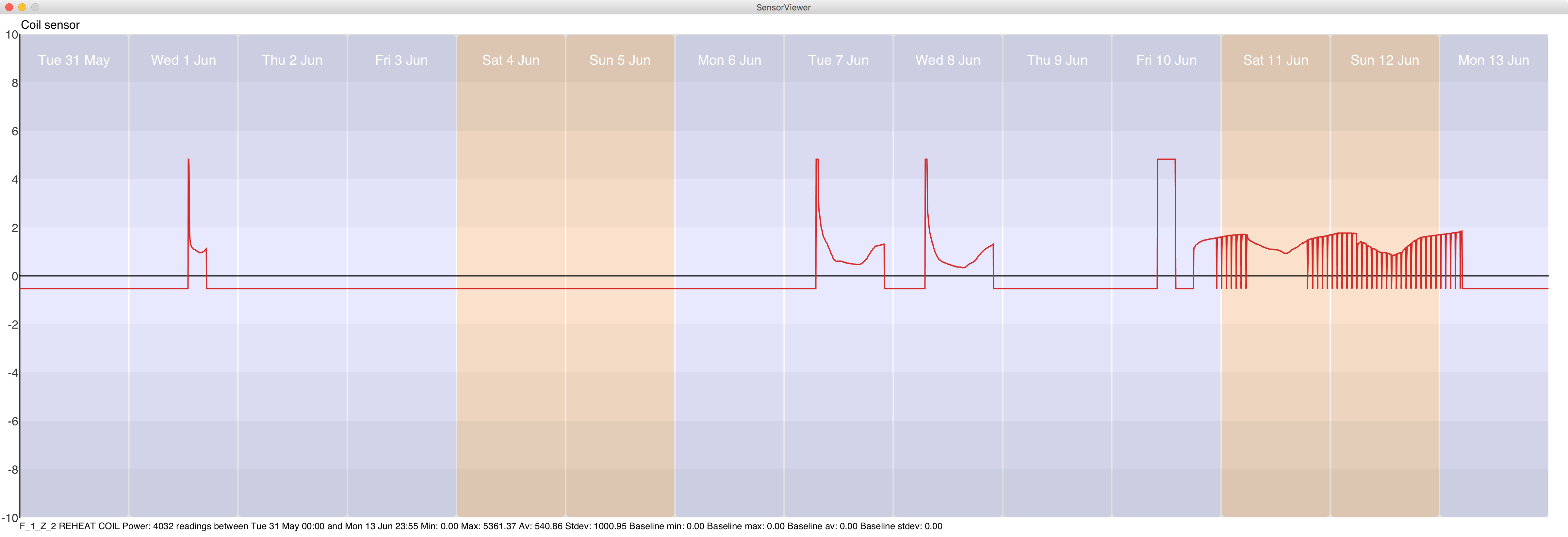
Figure 13 Reheat coil power sensor readings for floor 1 zone 2. (click image for full size)
The power sensor readings, especially the reheat coil power sensors provide more precision on the 7-8th June temperature and air anomalies. The spike in power for the coil at around 7am on both days represents the change from negative to positive temperature anomaly. There is also evidence of a spike in light power on floor 1 on Tuesday 31st.
MC2.3 — Describe up to ten notable anomalies or unusual events you see in the data. Describe when and where the event or anomaly occurs and describe why it is notable. If you have more than ten anomalies to report, prioritize those anomalies that are most likely to represent a danger or serious issue for building operation.
(i) Unusual Saturday Activity from Bramar and Strum
As described in section MC2.1, almost all employee activity occurs during weekdays only. Even late shift workers finish by midnight on Friday. There are four exceptions evident from the prox card timelines where card entries occur during weekend periods. Of particular note are the entries using the cards of Mat Bramar and Orhan Strum on Saturday 11th June between the periods of 8:30-11:30am (Bramar) and 9:00-13:00 (Strum) (See Figure 14). This is notable because not only do they intersect in time and space but they also occur just before the only weekend outbreak of Hazium gas (see MC2.4 below).
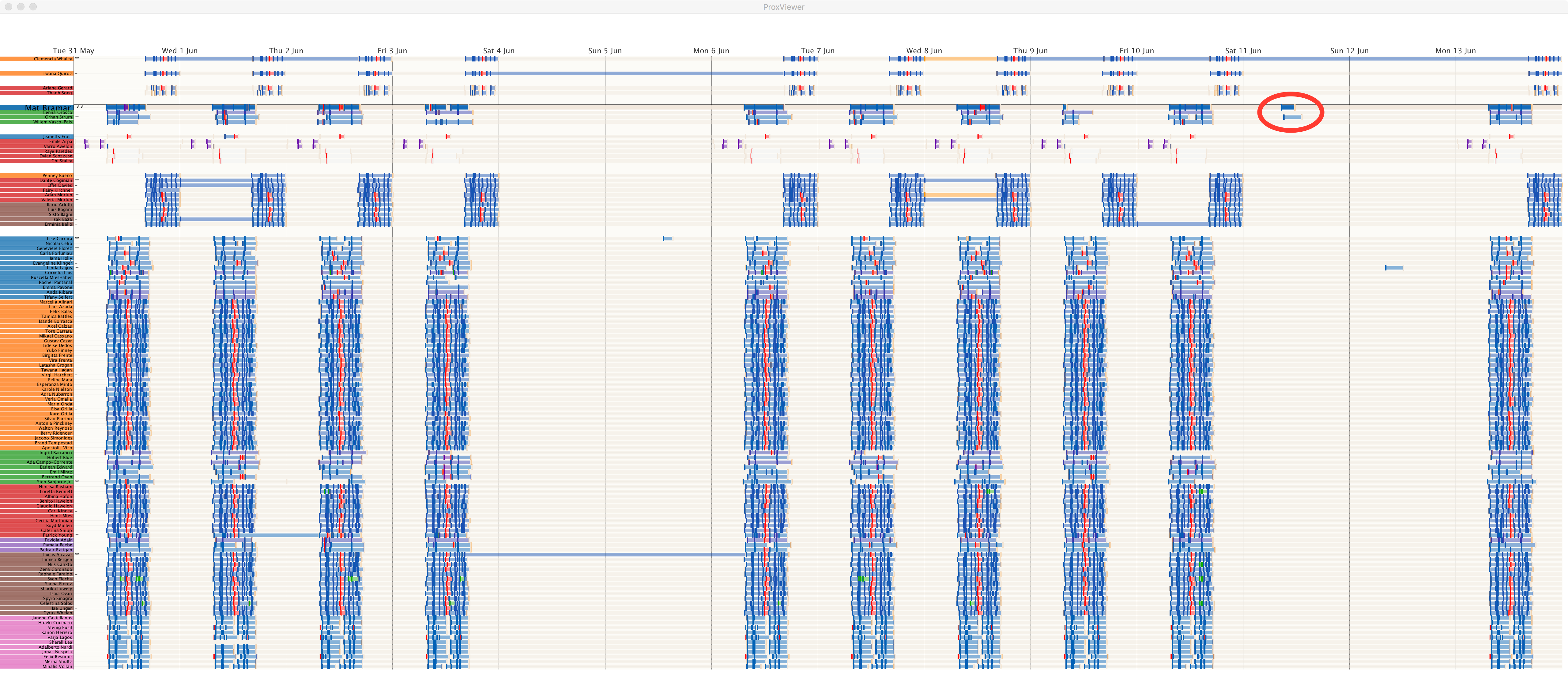
Figure 14 Prox card acitivity showing notable weekend behaviour of Mat Bramar and Orhan Strum. (click image for full size)
(ii) Multiple Card Issues for Geneviere Florez
Several employees have required a second issue of their prox card after losing their original, but only one employee – Geneviere Florez – has had 3 card reissues within the two week period. This may be due to carelessness on her part but it does raise a security concern especially as her administrative role on the executive floor may give access to confidential GASTech material. Of notable concern is that there is an unusual midnight prox card entry on Monday 6th into Tuesday 7th. This may not be Geneviere herself, but given her apparent carelessness with her prox cards, a lost card may have been picked up by someone else and used. It is also worth noting that this midnight period is a few hours before the major air/temperature anomaly described in section MC2.2 above.
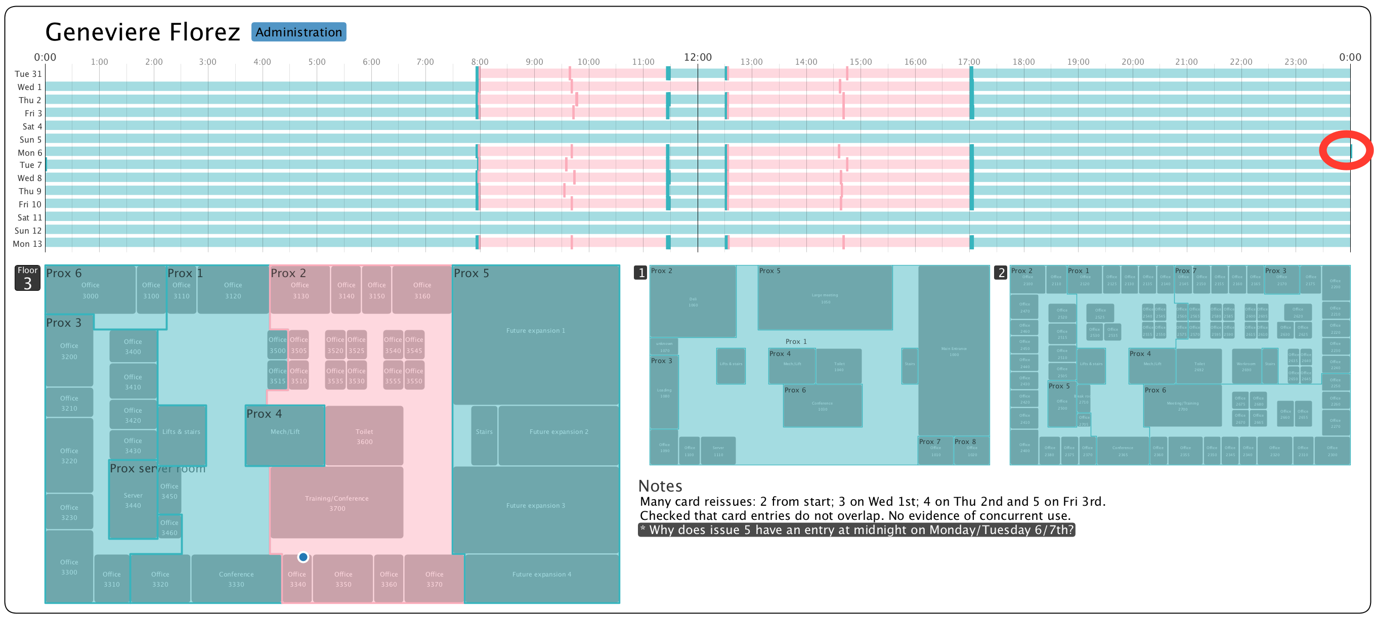
Figure 15 Geneviere Florez's prox entries showing unexpected midnight activity (click image for full size)
(iii) Midnight Activity for Sten Sanjorge Jr
CEO Sten Sanjorge Jr works long hours but usually between 7am and 6pm. However unusually his card shows an entry around midnight Wednesday 1st/Thursday 2nd June. This is unexpected and anomalous as there appear to be no other prox card entries in the 12 hours either before or after this entry.
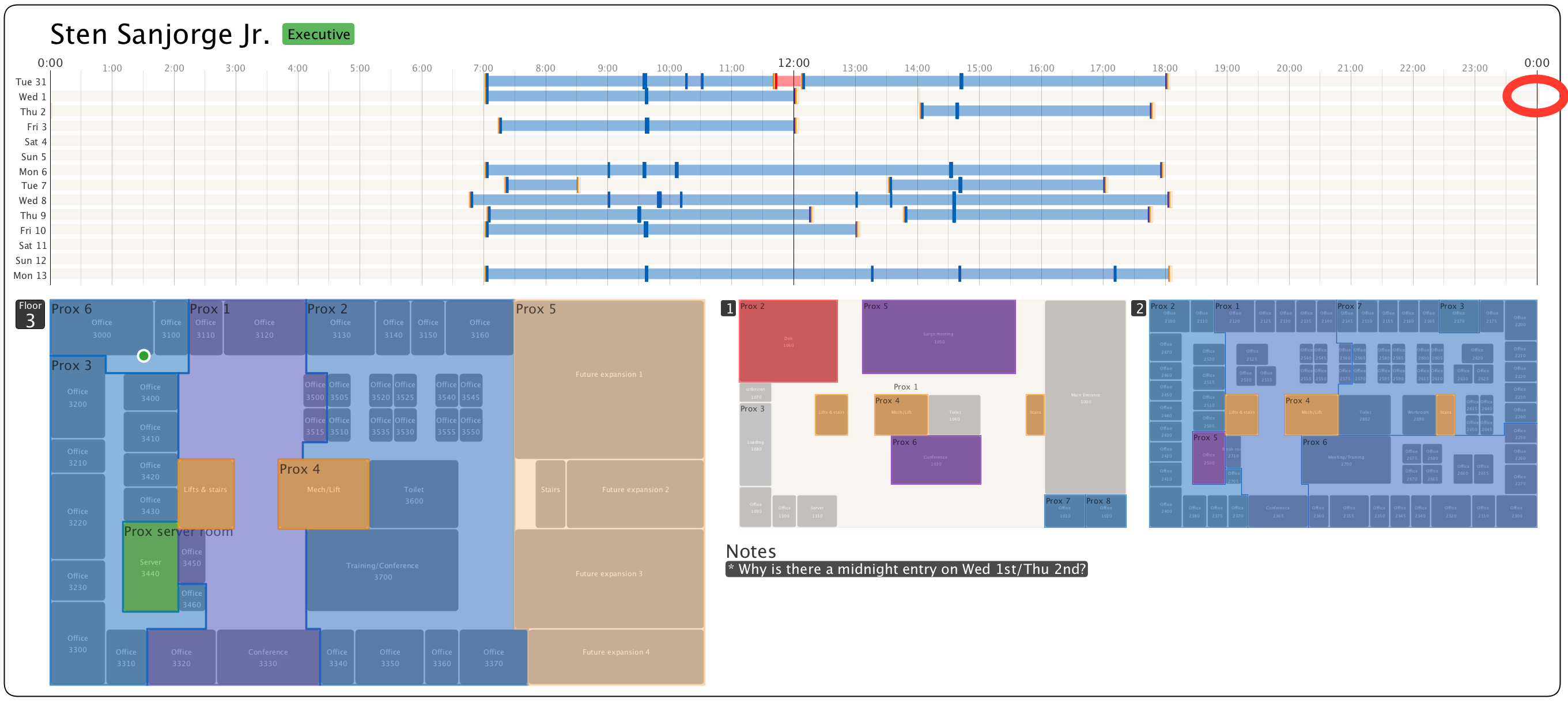
Figure 16 Sten Sanjorge Jr's prox entries showing unexpected midnight activity (click image for full size)
(iv) Air / Temperature problems on Tuesday 7th and Wednesday 8th June
This anomalous change in air temperature, carbon dioxide level and associated temperature regulation and heating equipment has been described in detail in section MC 2.2 above. The period is notable in that it is also coincides with other anomalous prox card patterns (described below).
(v) No building exit records for some staff especially at end of 31st May and 7th June
Most staff show evidence of leaving the building at the end of each day by a prox card entry in Prox Zone 1 on the ground floor of the GasTech HQ. The prox card timelines show where this does not occur, typically by an elongated bar spanning one or more night-time periods. There are four staff who show this lack of exit readings on the same evening at the end of Tuesday 31st May (Clemencia Whaley, Dante Coginian, Effie Davies and Isak Basa). Two of them are also in a group of four who do not show any exit readings at the end of Tuesday 6th June (Clemencia Whaley, Dante Coginian, Valeria Morlun and Adan Morlan) all of whom work the late shift usually finishing just before midnight. It is unusual for four instances of non prox exit to occur at the same time. Clemencia Whaley fails to show an exit from the building on six occasions in the two week period (see Figure 18) which suggests she is leaving the building unconventionally.
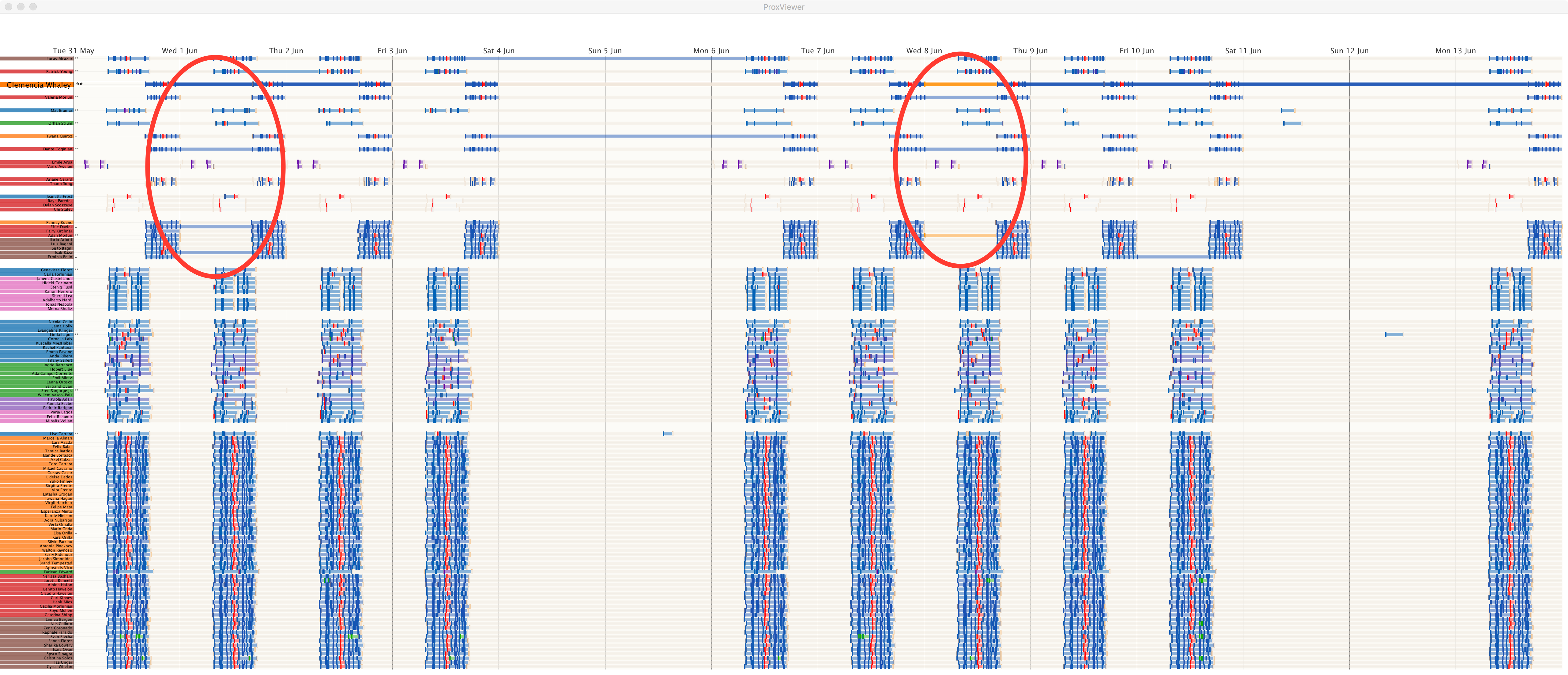
Figure 17 Staff showing no prox card exit from building on Tuesday 7th (click image for full size)
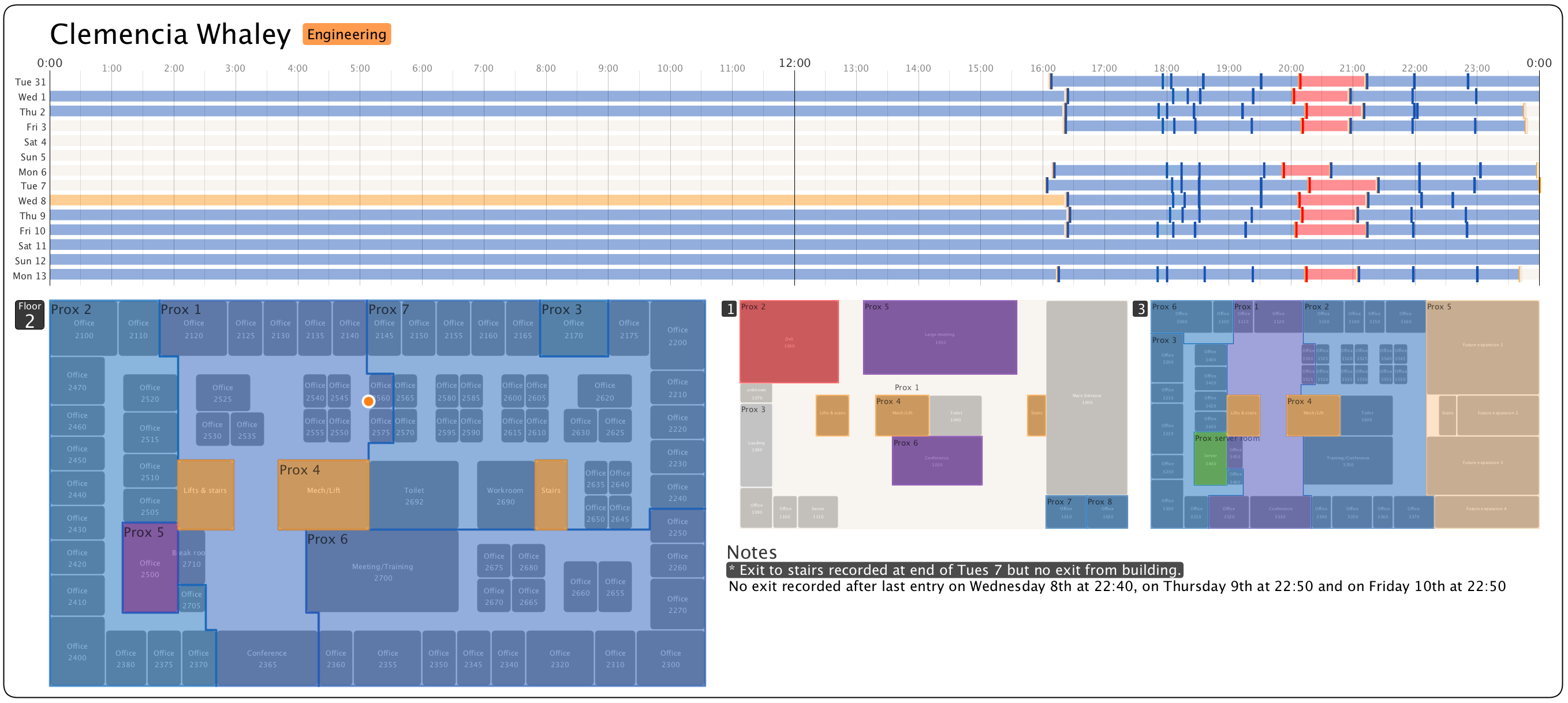
Figure 18 Clemencia Whaley's lack of exit prox card readings (click image for full size)
(vi) Other Unusual Weekend Activity
Similar to the anomalous weekend prox card readings for Bramar and Strum, there are two more cards that show non-weekday activity (visible in Figure 14 above). They are from Lise Carrera on Sunday the 5th of June and Linda Lagos on Sunday 12 June.
(vii) Staff Absences
Possibly not suspicious, but worthy of note are the absences of some staff for selected days. This may be due to sickness or planned absence but it would be worth checking with personnel records to confirm. Three staff appeared absent – Sherell Lea, Ingrid Barranco and Orhan Strum. Strum's absence in particular should be investigated given his unusual Saturday activity noted above.
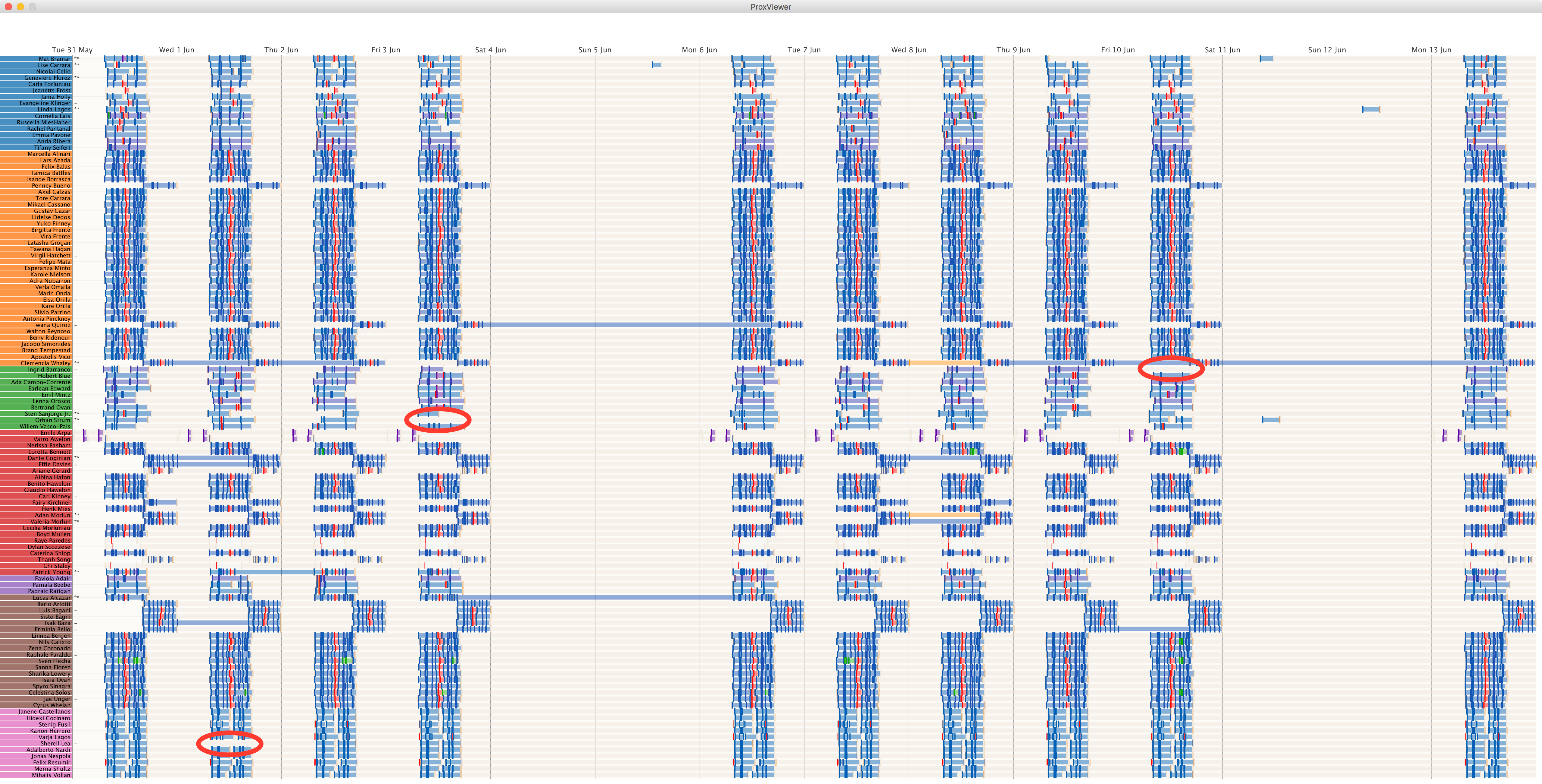
Figure 19 Staff absences (highlighted) with a working day showing no prox card activity (click image for full size)
MC2.4 — Describe up to five observed relationships between the proximity card data and building data elements. If you find a causal relationship (for example, a building event or condition leading to personnel behavior changes or personnel activity leading to building operations changes), describe your discovered cause and effect, the evidence you found to support it, and your level of confidence in your assessment of the relationship.
Temporal relationships between the prox card data and the building data can be seen by overlaying the sensor readings onto the same timelines of prox card entries.
(i) Strum, Bramar and the weekend Hazium event
The largest peak in Hazium concentration evident on all floors occurred on Saturday 11th June shortly after Mat Bramar left the building and around the time Orhan Strum also left (highlighted in Figure 20). Given weekend prox activity is highly unusual and the magnitude of the Hazium readings, this should be investigated further. The evidence for the association of the two events is strong, but a causal relationship is not yet established. However, this weekend Hazium event is the only one that occurs outside of the working week and Strum and Bramar are the only ones apparently present in the building. There is a possibility that their cards may have been used by someone else so independent evidence of their whereabouts should be sought.
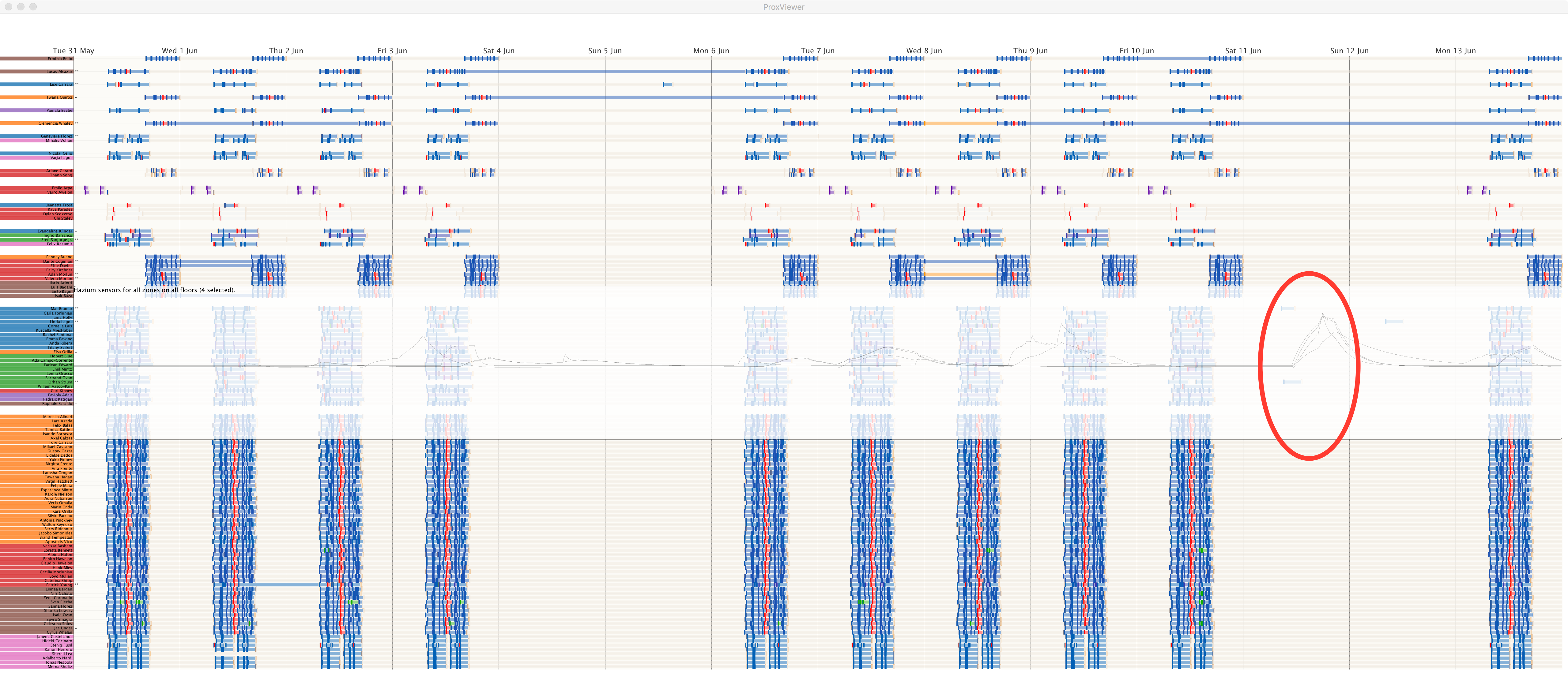
Figure 20 Hazium readings combined with prox card timelines. (click image for full size)
(ii) Hazium Events and Staff Health and Safety
It is evident from overlaying the Hazium readings with the prox readings (Figure 20 above) that there is a serious health and safety issue for employees of GASTech as the Friday 3rd, Tuesday 7th and Thursday 9th Hazium peaks all coincide with busy working periods in the same zones as the gas detection. Confidence in the co-location of the leaks and working staff is very high. Less certain is the health effects of the exposure as Hazium is a newly discovered hazard.
Of particular concern is the detection of Hazium in HVAC Zone 1 on Floor 3 as this is the CEO Sten Sanjorge Jr's office. The three peaks (green lines in Figure 21) in his office are precisely timed with him entering the room as can be seen by comparing them with his proximity line (5th line from the top in Figure 21). That Hazium was not detected in the adjacent HVAC zones of floor 3 at the same time suggests, with moderately high confidence, that he may have been the target of deliberate attempt to contaminate him with the gas.
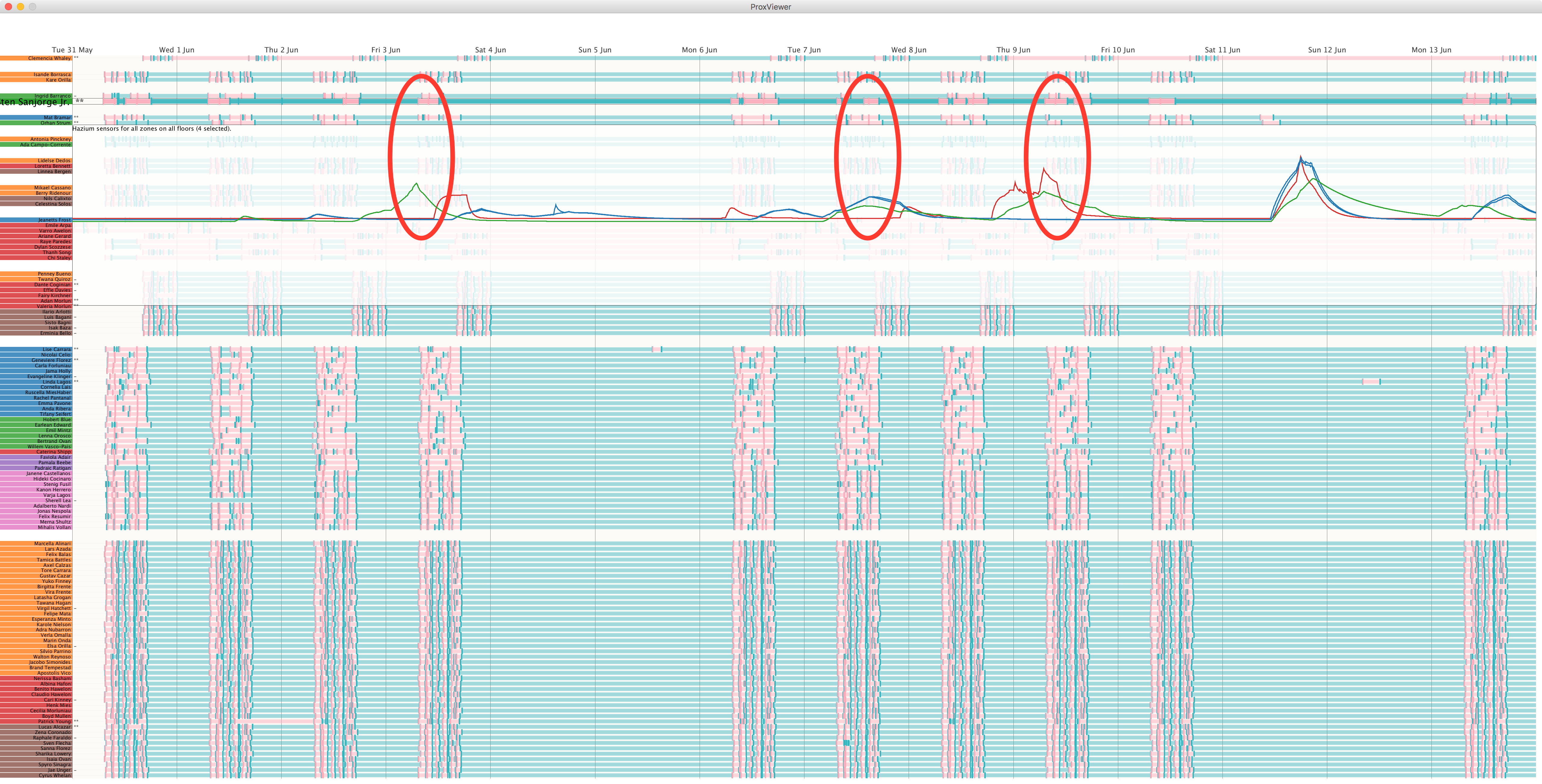
Figure 21 Hazium readings and Sten Sanjorge. (click image for full size)
(iii) General Association Between Building and Staff Activity
By showing all building sensor readings on the same timeline, the associations between the various sensors and staff activity during the day and over the two weeks is revealed. There are clear differences between the building activity during working and non-working hours (as we might expect). Less expected is the difference between Saturday and Sunday sensor activity despite there being no difference in staff presence over the two weekend days. This may simply be due to differences in the recovery period following a Friday and the preparation period in anticipation of Monday.
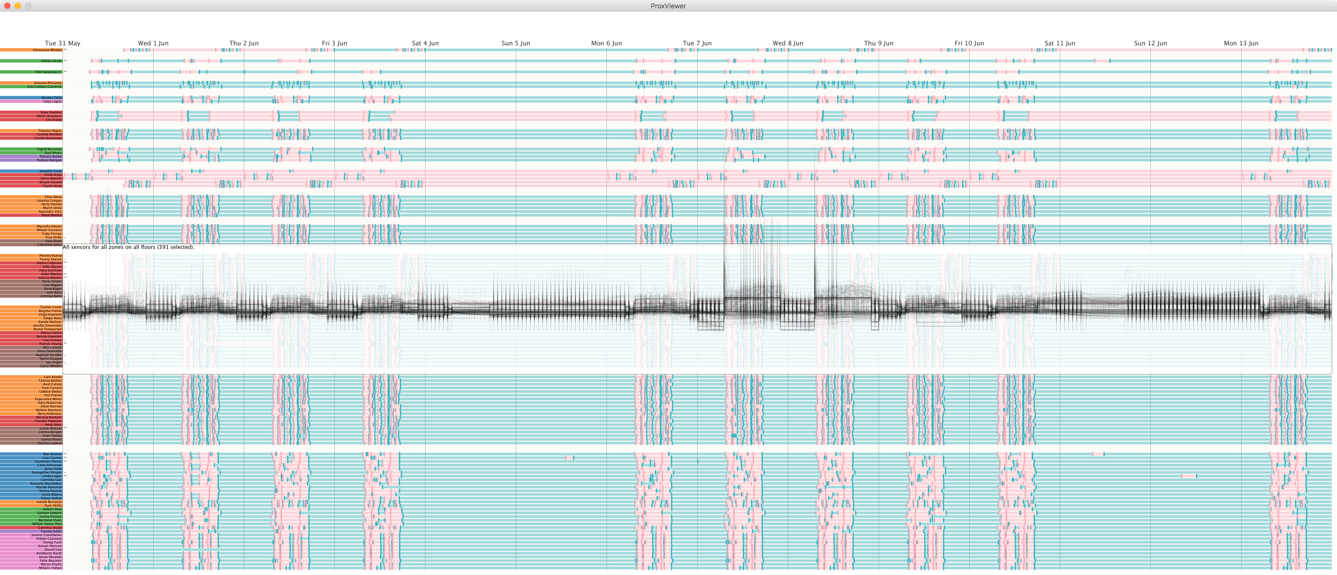
Figure 22 All building readings combined with prox card timelines. (click image for full size)
(iv) Temperature Anomaly and Staff Activity
The temperature and air anomaly of around the 6th and 7th of June can be seen in relation to staff activity (Figure 23). In particular is is evident that the first drop in temperature sensor readings occurs in the early hours of Tuesday 7th June shortly after the late shift Information Technology staff (shown in brown) had left the building. The following spike in temperature sensor readings occurred as staff started to enter the building from 7am. A similar pattern was repeated on the 8th June although these sensors returned to normal working levels shortly after midday on the 8th.
It might be expected, given the significant temperature rise (see Figure 11a above), that we would expect a change of staff behaviour in response to the uncomfortable conditions, especially on Floor 3 where temperature changes were most obvious. Examining the locations of the executive and admin staff located on this floor, there is no obvious change in behaviour during those two days.
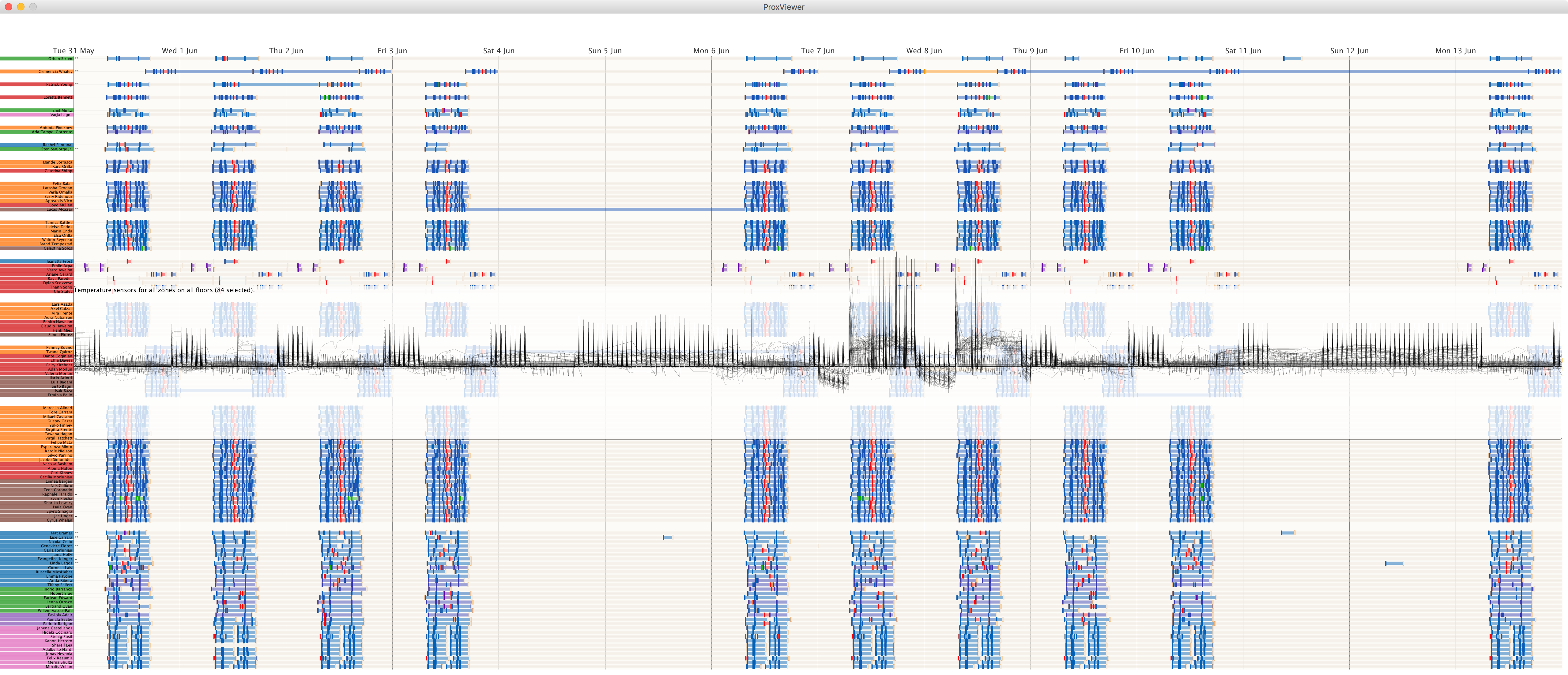
Figure 23 Temperature sensor readings combined with prox card timelines. (click image for full size)